The echo noise created by return loss is relatively easy to understand. This technical brief uses channel modeling techniques to prove that return loss also directly affects the quality of the transmitted signal and that impedance-controlled patch cords can improve any high performance LAN.
It has become well known that return loss is an important parameter for cabling used in bidirectional signaling. (See “Why Is Return Loss Important? ” “The Hidden Cost of High Speed Networks,” and “Performance of Premise Wiring Systems at Extended Frequencies” at Technology Briefs). It is less well known that poor return loss can affect any high-speed network, even those employing unidirectional signaling. In this paper we will show how return loss or, more accurately, impedance mismatches impact the transmission of digital signals and thus affect any high speed local area network.
An important noise source in base band signaling is inter-symbol interference or ISI. This occurs when the received pulses or symbols spread into adjacent pulses or symbols. Pulses spread as a result of cable losses that vary or change with frequency. The energy in the input signal disperses or spreads in time as the pulse moves down the cable. Higher speed networks have narrower pulses with higher frequency components and require a larger bandwidth. They are also more susceptible to dispersion and ISI. 1000Base-T modeling on Cat 5 cabling has shown that ISI will be 104mV rms or approximately two orders of magnitude greater than NEXT and FEXT at the input of the receiver. (Source: Sailesh Rao, Level One Communications. Presentation to TIA TR 41.8 Committee, November 17, 1998.) Multi-level signaling schemes also demand a higher signal-to-noise ratio in order to achieve acceptable bit error rates. The residual ISI budgeted for Gigabit Ethernet is only 2.1mV rms in order to meet the desired signal to noise ratio and bit error rate requirements for its five level signaling scheme. (Rao, 1998)
Return loss and ISI are related by insertion loss (attenuation) deviation. Impedance mismatches in the cabling cause reflections that are seen as lower return loss. (Note: throughout this paper, low return loss means low loss to the reflection or smaller negative numbers in dB; high return loss means high loss to the reflection or larger negative numbers in dB. High return loss is desirable.). Because the power is reflected rather than transmitted, the output power is reduced. Although this is often called attenuation deviation, attenuation by definition does not include reflected losses. Attenuation only includes the material (resistive and dielectric) losses of the cable. Typically, in the LAN industry attenuation is measured and specified in a 100 ohm system, therefore both reflected and material losses are included in the measurement. The difference between attenuation and insertion loss is important in the calculation of the transfer function of the cabling.
Attenuation is part of the transfer function of the cabling system. The transfer function is the ratio of the output voltage of the cabling to its input voltage. For cabling with no impedance mismatches (that is, with very high return loss) it is:
H(f)=Vout/ Vin =ej(ja(f)+b(f))l (1)
Vout is voltage out of the cabling
Vin is voltage into the cabling
a (f) is attenuation in Nepers
b (f) is propagation constant of cabling
l is length in meters
When impedance mismatches are present (cabling with lower return loss), another term must be included in the transfer function to account for the signal loss due to reflection:
H(f)=Vout/ Vin = (1-r(f))ej(ja(f)+b(f))l (2)
r (f) is the voltage reflection coefficient.
1-r (f) is t (f), the voltage transmission coefficient.
If all components in a channel are close to 100 ohm impedance, t (f) is close to 1 and has little effect on the transfer function of the channel.
To determine the effects of return loss on data transmission, three connector channel models were created using standard transmission line modeling. Figure 1 illustrates the physical description of the channel. Model A had no impedance mismatches (very high return loss), Model B had small impedance mismatches (<2 ohms difference in cable and return loss 18 dB @ 100 MHz connectors) and Model C had large impedance mismatches (patch cords of 108 ohm, 88 ohm; 88 ohm; horizontal cable, 108 ohm; and one connector at 10 dB and two connectors at 18 dB). Model C was designed to not pass Cat 5e channel requirements between 10 MHz and 30 MHz.
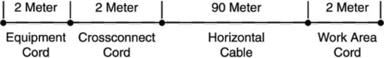
Fig. 1. Channel model configuration
The transfer function for each model was determined using equation (2). For Model A t (f) is equal to 1. Figure 2 is a plot of the transfer function for channel Model A (very high return loss). Note the smooth shape of the curve. Figure 3 is a plot of the transfer function for Model B (high return loss, t (f) close to 1). Note that the curve is similar to figure 2 but has some roughness. Figure 4 is the transfer function for Model C (low return loss, t (f) less than 1). Note that the shape is similar to figure 2 and figure 3 but has more variation with frequency. We expect the effect that channel Model C has on a pulse will be different from that of channel Model B.
Fig. 2. Model A transfer function
Fig. 3. Model B transfer function
Fig. 4. Model C transfer function
In order to determine the effect of the different transfer functions on a signal, a number of calculations need to be performed because the signals are time based and cabling parameters are all frequency based. The following flow chart (Fig. 5) is a summary of the method used to predict the output of each channel model for a given input.
Fig. 5. Flow chart of calculations
To convert from time domain to frequency domain, a Fast Fourier Transform (FFT) was used. The FFT calculation used a sampling frequency of 1GHz, 8,000 data points and no data windowing. To convert from frequency domain to time domain, an inverse FFT was used. The routines used were from MathCad 7 Professional but they can be found in many mathematical packages. To convert from time domain to frequency domain, a Fast Fourier Transform (FFT) was used. The FFT calculation used a sampling frequency of 1GHz, 8,000 data points and no data windowing. To convert from frequency domain to time domain, an inverse FFT was used. The routines used were from MathCad 7 Professional but they can be found in many mathematical packages.
The input pulse used is shown in figure 6. Rise time was approximately 3.4 ns and the pulse width was 8 nS. Although this represents a signal rate (125 MHz) and rise time similar to some current high speed networks, no attempt was made to meet the specific requirements of any network protocol. Using the method outlined above, output pulses were produced using Model A (no return loss), Model B (high return loss), and Model C (low return loss) transfer functions. Figure 7 is the output of Model A. Note that the pulse has spread out due to the attenuation of the cabling. Because the pulse has spread out of the 8 nS window it will interfere with adjacent pulses causing ISI. Figure 8 is the output from channel Model B. Note that the output pulse is very similar to channel Model A output. This is expected because the transfer function of Model B was very similar to Model A. Figure 9 is the output from channel Model C. Note the lobe in the pulse edge, which is not present in figure 7 or figure 8. This distortion is caused by the deviation or roughness of the transfer function from the ideal smooth curve in figure 2.
Fig. 6. Input signal
Fig. 7. Model A output pulse
Fig. 8. Model B output pulse
Fig. 9. Model C output pulse
To determine the significance of the lobe in the output from channel Model C, eye patterns for Model B and Model C were generated using a data pattern comprised of 3-level pulses. This is similar to 100Base-T signaling, however the pattern may not be a permitted sequence in 100Base-T encoding. The size of the eye opening in an eye pattern represents the signal quality at the input to the receiver. The eye patterns were generated by inputting the random data pattern into the transfer function exactly as was done for a single pulse, then shifting the output in time so that many pulses are in the same interval.
Figure 10 is the eye pattern for channel Model B, which has high return loss and small impedance mismatches. Note the size of the opening in the shaded area. Using the same data pattern, the eye pattern in figure 11 was produced using channel Model C, which had low return loss and high impedance mismatches. Note the smaller size of the opening in the shaded area caused by the lobe in the output pulses. This is increased ISI.
Fig. 10. Eye pattern, Model B
Fig. 11. Eye pattern, Model C
ISI can be improved by adding an equalizer to the channel. In the simplest form, an equalizer will have a transfer function inverse to the cabling transfer function, producing a net flat response for the channel. An equalizer with a smooth response will not completely remove the extra distortion in the pulse caused by impedance mismatch, which will lead to higher residual ISI. An equalizer with a smooth response would be more effective in channel Model B than in channel Model C. As noted earlier, the budget for residual ISI can be quite small in complex signaling schemes.
In order to determine the effect of patch cords on the eye pattern and data transmission, the parameters for channel Model C patch cord were replaced with the parameters for channel Model B patch cords. The connector and horizontal cable parameters were not changed. This is equivalent to replacing only the patch cords in an installed channel and not replacing any permanently installed components. Using the same data pattern as before, an eye pattern was produced for this new version of channel Model C and plotted in figure 12. Note that the eye openings are very similar to the eye openings for channel Model B. This result shows that patch cords with tight impedance tolerance have a significant effect improving the quality and speed of high frequency data transmission.
Fig. 12. Eye pattern, Model C with good patch
In this paper we have shown that a channel with low return loss (large impedance mismatches) will not perform as well as a channel with high return loss (small impedance mismatches) even when the network is not a bidirectional network such as Gigabit Ethernet. Large impedance mismatches degrade signals in unidirectional networks such as those using 100Base-T or ATM. In a bidirectional Gigabit network return loss degrades performance twice: first, through reflected power at the near end and, second, through increased ISI at the far end. We have therefore shown that high quality patch cord can be used to improve channel return loss and improve noise margins in any high performance channel.
To comment on this paper, send an e-mail message to engineering@quabbin.com.