Quabbin Wire & Cable tested the performance of LAN premise systems at extended frequencies. This article describes that program and the conclusions. The surprising result was that system return loss and impedance stability are critically important at frequencies beyond 100Base-T Ethernet.
Background to the test program
As background, understand that new and faster LAN protocols have been developed and are now commercially available. What are these new LAN protocols and what is their impact? First, many network users are beginning to install 1000Base-T, or Gigabit Ethernet. This protocol uses all four pairs in the cabling system instead of two pairs that are used for 10Base-T and 100Base-T networks. Each pair employs full duplex signaling, simultaneously sending and receiving data. This increased speed and signaling complexity stresses premise networks more than the previous, slower versions of Ethernet did.
Impedance becomes unstable at high frequencies
Years ago Quabbin tested a very simple network that consisted of three meters of patch cord and 90 meters of horizontal cable and found that above 70 MHz the network’s impedance stability broke down.
Pair Test Data for Simple Network
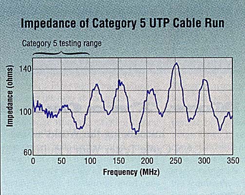
Figure 1. Substituting high performance patch cable stabilized the impedance beyond 70 MHz.
Figure 1 shows that the network was relatively stable at very low frequencies, but as the frequencies approached 100 MHz, the impedance began extreme oscillations. An ideal network should be very stable around the 100 ohm impedance line.
During the testing, Quabbin discovered that if you substituted a high performance patch cord that used higher quality stranded conductor cable assembled with the same connector plugs, the network’s impedance stability became much better. How could such a short patch cord assembly have such a dramatic effect on a much longer network?
This earlier test also raised questions as to the importance of cabling impedance stability in a high frequency network. Manufacturers know that a cable pair’s impedance varies very slightly along its length. This is due to small variations in manufacturing, such as concentricity, diameter, quality of twisting and wall thicknesses. These small impedance variations along each pair create signal losses due to reflections of the energy transmitted along the pair. These losses are more significant at higher frequencies because, as the signal wavelengths become shorter, small variations become more visible in the network. Impedance stability at low frequencies is relatively easy to achieve, but gets much more difficult as frequencies increase. Higher performance cables are manufactured with very tight manufacturing tolerance controls. This stabilizes their impedance and minimizes the reflected losses in the network.
System return loss is also important
Return loss is another critical measurement for a premise system. Return loss measures all the relative reflected power lost in a network. For a system designer, low return loss is the sign of a quality system and is measured from the ideal 100 ohm impedance target for the network.
Network return loss becomes much more important at frequencies above those of 100Base-T. A network with high return loss also exhibits unstable attenuation and phase delay. Most active components in a network use equalization circuits to stabilize network signaling. This is done by integrated circuits that compensate for the attenuation of the network. If the attenuation is unstable and doesn’t follow a smooth curve, equalization becomes very difficult and the chips very expensive. High return loss also creates what electronic engineers refer to as “jitter” in the signaling. This is due to delay and distortions of the digital signals. It also affects the signal-to-noise ratio of the network, which is very important for efficient, full duplex signaling. Last, analog video signals will be subject to “ghosting”. You will see multiple or flickering images, due to the timing problems that occur when return loss gets out of control. Video transmission is important for multimedia, video conferencing, and some Industrial Ethernet applications.
The new premise system test setup
To measure the high frequency performance of networks for the new program, Quabbin set up equipment diagramed here as Figure 2.
Test Setup to Measure Premise System Performance
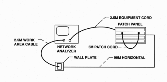
Figure 2. The equipment arrangement closely approximates a “worst case” installed channel.
You can see from the diagram that a network analyzer was connected to 2.5 meters of patch cord that represented work area cabling. This was terminated through a wall plate to a 90 meter run of horizontal cable. The horizontal cable was connected to a patching system, that would normally be in the wiring closet. A flexible patch cord was installed on the patch panel. The last portion of the network is another 2.5 meters of flexible equipment cord which would normally go to a hub, bridge, or router, but for the test it was terminated back to the network analyzer. Notice that Quabbin was able to test both directions through the network.
Quabbin discussed this test program with many manufacturers of premise hardware and invited them to participate. They were asked to supply their best connectors, patching systems and other hardware. Impedance, return loss and other data that relates to system performance was measured for each manufacturer. The goal was to learn how systems performed and to share the data with individual manufacturers.
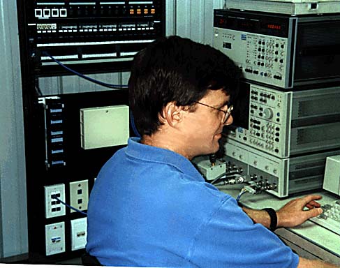
Figure 3. View of actual test set-up.
Figure 3 is a photograph of the test setup. In the left background is a vertical rack with equipment mounted in it. At the top are the patch panel devices. Each manufacturer was given one slot in the rack where its patch devices were mounted. At the bottom of the rack the wall plate hardware can be seen. In the right background is the network analyzer. The connections to the analyzer can be seen below, and the PC that is driving the system is in front of the operator. The cabling was connected to the network analyzer on one side through a connector, to a high frequency balun and then into the network analyzer. On the other end of the network the cable was pinned out to a connector and terminated to a precision 100 ohm load. For a detailed description of the test components, refer to Appendix A .
System test results
Quabbin evaluated over 35 different premise hardware systems. Almost every major manufacturer was included. First, we learned that there is a significant difference between hardware systems, especially above 50 MHz. Also, it was discovered that patch cord has a very large effect on the system’s performance, especially return loss and impedance. Third, all premise systems, regardless of their quality, benefit from using the best available patch cable. It was unexpected to discover the great importance that patch cord has on a high frequency network.
Actual test data from this program is shown below. For obvious reasons, the specific results for each system tested were shared only with that manufacturer. Impedance and return loss are charted for two systems—a relatively high performance system and a relatively low performance system. The same 90 meter high performance horizontal cable run was used in all tests. The only change to each premise system was to exchange the lengths of patch cord. In one case, Quabbin used cords assembled using a minimum performance Category 5 cable, and in the other case patch cord was assembled using Category 6 patch cable. In both cases, the cords utilized the same high performance Category 6 plugs from AMP. Thus, the only variables in this data were the premise hardware and the quality of the cable used to assemble the 2.5 meters of patch cord.
Figure 4 shows a high performance hardware system with the lower quality patch cable. Impedance stability, which ideally should be close to the 100 ohm target line, begins to break down at about 50 MHz. You see wide variations in the measured impedance for every pair.
High Performance Hardware/Low Performance Patch Cable, Wall Plate End
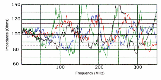
Figure 4. System stability breaks down at about 50 MHz.
When the same high performance hardware system was tested with a Category 6 patch cord (Figure 5), you see that the impedance became remarkably smoother. It is relatively flat out through 350 MHz.
High Performance Hardware/DataMax 6 Patch Cable, Wall Plate End
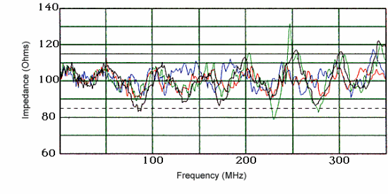
Figure 5. System is much smoother through 350 MHz.
The next chart (Figure 6) shows the return loss for this high performance system using marginal patch cords. The darker line that is drawn at 25 db return loss out to 70 MHz and then decreases, represents a reference target. It is based on what the test data showed as an achievable level for return loss for one of the best systems. Quabbin arrived at this target level after testing many systems.
High Performance Hardware/Low Performance Patch Cable (Wall Plate End)
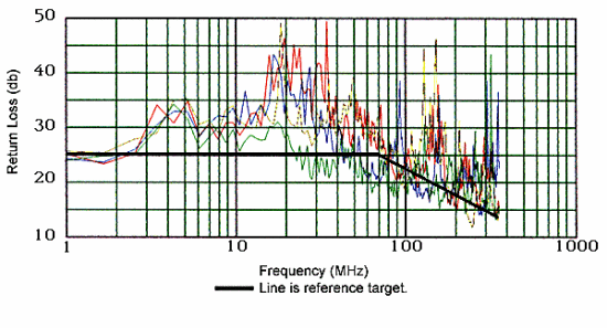
Figure 6. Return Loss is good to 20 MHz.
The return loss for this same system with superior patch cords meets the reference target level, as is illustrated in Figure 7. It was completely unexpected that a better patch cord could have such an impact on a network.
High Performance Hardware/DataMax 6 Patch Cable (Wall Plate End)
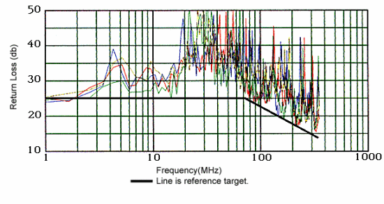
Figure 7.
The next two figures show the impedance stability of a lower performance hardware system. Figure 8 illustrates the performance with the low performance patch cable. You see that the impedance begins to break down around 30 MHz. Taking this same low performance hardware system and installing high performance patch cords improves it. This can be seen in Figure 9. Cable impedance is relatively smooth out to about 100 MHz.
Low Performance Hardware/Low Performance Patch Cable (Wall Plate End)
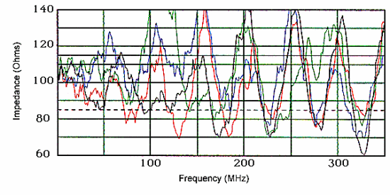
Figure 8. Impedance variation increases at 30 MHz.
Low Performance Hardware/DataMax 6 Patch Cable (Wall Plate End)

Figure 9. Impedance is much smoother out to 100 MHz.
Measuring return loss for the lower quality system combined with the lower performance patch cable illustrates good performance only to 10 MHz. Beyond 10 MHz return loss deteriorates rapidly, as can be seen in Figure 10. However, the return loss for this system can be significantly improved by changing the patch cords. In Figure 11 you see performance above the target level to about 50 MHz instead of 10.
Low Performance Hardware/Low Performance Patch Cable (Wall Plate End)
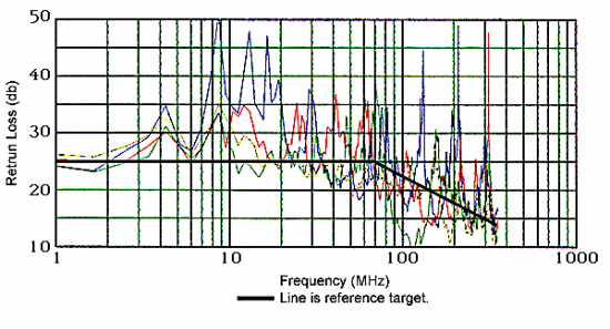
Figure 10. Return Loss is good to 10 MHz.
Low Performance Hardware/DataMax 6 Patch Cable (Wall Plate End)
Figure 11. Return Loss is good to 50 MHz.
When Quabbin Wire & Cable began measuring return loss (RL) of networks for this test program, it was a metric that had not yet been quantified by the TIA’s LAN industry standards. However, RL has since proven to be a critical new measurement quantifying network performance. Low system RL is vital to assure lower bit error rate, more system throughput and higher operational margin when transmitting the newer high frequency or bidirectional protocols. For more information on RL, refer to the technical article and
High Performance Hardware/DataMax 6 Patch and Horizontal (4m + 90m)
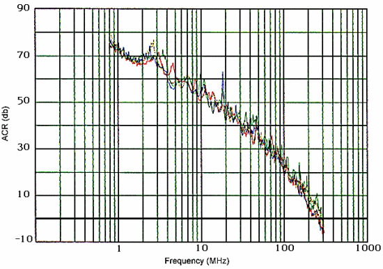
Figure 12
Conclusions from the test program
What did this system testing accomplish? Test data from this program directly influenced the limit lines now defined for Category 6 channels and the design parameters for several hardware systems. These performance levels were defined using the data and technology that flowed from this program.
This program also demonstrated component stability. Quabbin found that some manufacturers have wall plates that perform much better than their patching system and vice versa. Others have extremely good control on their entire system. Testing systems showed how well components are matched. If components do not closely match the 100 ohm system impedance target, they will not perform well as a system. Quabbin also proved that you have to look at end-to-end performance of a system. It is not sufficient to look at the performance of a component. A marginal component can have a huge negative effect on the entire system at high frequencies.
This program showed that systems with the best performance have the most margin and will survive some installation abuse. Subtle changes or small mistakes in terminating a connector or connecting the system were immediately apparent. The test program demonstrated that it is possible to assemble premise systems which will support protocols that require the very best high frequency performance. Last, the test program clearly demonstrated that a high performance patch cord is critical in order to assure the optimum high frequency performance of any premise hardware system.
What are the bottom line conclusions drawn from this test program? If you install, specify, or own a premise system, you should be very interested in the data you have just seen. It shows a new way to evaluate system performance using return loss. You now have some new questions to ask, and data to ask for, when you compare premise systems. But most important, patch cords must never again be considered an insignificant or “throw away” part of a network. A patch cord can make or break network performance. In many cases it is the most significant component. What are the bottom line conclusions drawn from this test program? If you install, specify, or own a premise system, you should be very interested in the data you have just seen. It shows a new way to evaluate system performance using return loss. You now have some new questions to ask, and data to ask for, when you compare premise systems. But most important, patch cords must never again be considered an insignificant or “throw away” part of a network. A patch cord can make or break network performance. In many cases it is the most significant component.
Enhanced system performance is available now. Specify and use premise systems that provide the best high frequency performance and insure that performance by using patch cords assembled with DataMax 6 flexible cable.
To comment on this paper, send an e-mail message to engineering@quabbin.com.